Nonlinear Regression
From Linear Regression to Nonlinear Regression
Given an arbitrary set of point \(\{(X_{i1},\dots, X_{in}, Y_i): i=1,\dots,m\}\) and an arbitrary norm \(\|\cdot\|\), a linear regression, \(\ell_{\|\cdot\|}\), with respect to the norm corresponds to a tuple of numbers \((a_1, \dots, a_n, b)\) such that
is minimized. Generally the norm is taken to be a wighted Euclidean norm. Then the association \(\ell_{\|\cdot\|}(x_1,\dots,x_n)=\sum_{j=1}^n a_i x_i + b\) provides an approximation for \(Y_i\)’s with respect to \(\|\cdot\|\).
Suppose that a set of basic functions, \(B=\{f_0,\dots, f_p\}\), a set of data points \(X = \{(X_i, Y_i) : i=1,\dots, m\}\), and a norm \(\|\cdot\|\) are given. A nonlinear regression, \(\mathcal{R}_B\), based on \(B\) and \(\|\cdot\|\) corresponds to a tuple \(a_0,\dots, a_p\) such that
is minimized.
Define a transformer
Then it is clear that \(\mathcal{R}_B(x) = \ell_{\|\cdot\|}\circ T_{B}(x)\).
Orthonormal system of functions
Let X be a topological space and \(\mu\) be a finite Borel measure on X. The bilinear function \(\langle\cdot,\cdot\rangle\) defined on \(L_2(X, \mu)\) as \(\langle f, g\rangle = \int_X fg d\mu\) is an inner product which turns \(L_2(X, \mu)\) into a Hilbert space.
Let us denote the family of all continuous real valued functions on a non-empty compact space X by \(\textrm{C}(X)\). Suppose that among elements of \(\textrm{C}(X)\), a subfamily A of functions are of particular interest. Suppose that A is a subalgebra of \(\textrm{C}(X)\) containing constants. We say that an element \(f\in\textrm{C}(X)\) can be approximated by elements of A, if for every \(\epsilon>0\), there exists \(p\in A\) such that \(|f(x)-p(x)|<\epsilon\) for every \(x\in X\). The following classical results guarantees when every \(f\in\textrm{C}(X)\) can be approximated by elements of A.
Let \((V, \langle\cdot,\cdot\rangle)\) be an inner product space with \(\|v\|_2=\langle v,v\rangle^{\frac{1}{2}}\). A basis \(\{v_{\alpha}\}_{\alpha\in I}\) is called an orthonormal basis for V if \(\langle v_{\alpha},v_{\beta}\rangle=\delta_{\alpha\beta}\), where \(\delta_{\alpha\beta}=1\) if and only if \(\alpha=\beta\) and is equal to 0 otherwise. Every given set of linearly independent vectors can be turned into a set of orthonormal vectors that spans the same sub vector space as the original. The following well-known result gives an algorithm for producing such orthonormal from a set of linearly independent vectors:
Note
Gram–Schmidt
Let \((V,\langle\cdot,\cdot\rangle)\) be an inner product space. Suppose \(\{v_{i}\}^{n}_{i=1}\) is a set of linearly independent vectors in V. Let
and (inductively) let
Then \(\{u_{i}\}_{i=1}^{n}\) is an orthonormal collection, and for each k,
Note that in the above note, we can even assume that \(n=\infty\).
Let \(B=\{v_1, v_2, \dots\}\) be an ordered basis for \((V,\langle\cdot,\cdot\rangle)\). For any given vector \(w\in V\) and any initial segment of B, say \(B_n=\{v_1,\dots,v_n\}\), there exists a unique \(v\in\textrm{span}(B_n)\) such that \(\|w-v\|_2\) is the minimum:
Note
Let \(w\in V\) and B a finite orthonormal set of vectors (not necessarily a basis). Then for \(v=\sum_{u\in B}\langle u,w\rangle u\)
Now, let \(\mu\) be a finite measure on X and for \(f,g\in\textrm{C}(X)\) define \(\langle f,g\rangle=\int_Xf g d\mu\). This defines an inner product on the space of functions. The norm induced by the inner product is denoted by \(\|\cdot\|_{2}\). It is evident that
which implies that any good approximation in \(\|\cdot\|_{\infty}\) gives a good \(\|\cdot\|_{2}\)-approximation. But generally, our interest is the other way around. Employing Gram-Schmidt procedure, we can find \(\|\cdot\|_{2}\) within any desired accuracy, but this does not guarantee a good \(\|\cdot\|_{\infty}\)-approximation. The situation is favorable in finite dimensional case. Take \(B=\{p_1,\dots,p_n\}\subset\textrm{C}(X)\) and \(f\in\textrm{C}(X)\), then there exists \(K_f>0\) such that for every \(g\in\textrm{span}(B\cup\{f\})\),
Since X is assumed to be compact, \(\textrm{C}(X)\) is separable, i.e., \(\textrm{C}(X)\) admits a countable dimensional dense subvector space (e.g. polynomials for when X is a closed, bounded interval). Thus for every \(f\in\textrm{C}(X)\) and every \(\epsilon>0\) one can find a big enough finite B, such that the above inequality holds. In other words, good enough \(\|\cdot\|_{2}\)-approximations of f give good \(\|\cdot\|_{\infty}\)-approximations, as desired.
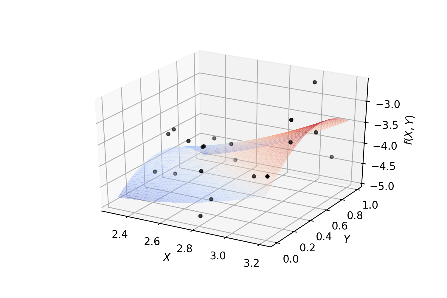
Example. Polynomial regression on 2-dimensional random data:
from mpl_toolkits.mplot3d import Axes3D
from matplotlib import cm
import matplotlib.pyplot as plt
import numpy as np
from GeneralRegression.NpyProximation import HilbertRegressor, Measure
from GeneralRegression.extras import FunctionBasis
def randrange(n, vmin, vmax):
    '''
    Helper function to make an array of random numbers having shape (n, )
    with each number distributed Uniform(vmin, vmax).
    '''
    return (vmax - vmin)*np.random.rand(n) + vmin

# degree of polynomials
deg = 2
FB = FunctionBasis()
B = FB.poly(2, deg)
# initiate regressor
regressor = HilbertRegressor(base=B)
# number of random points
n = 20
fig = plt.figure()
ax = fig.add_subplot(111, projection='3d')
for c, m, zlow, zhigh in [('k', 'o', -5, -2.5)]:
    xs = randrange(n, 2.3, 3.2)
    ys = randrange(n, 0, 1.0)
    zs = randrange(n, zlow, zhigh)
    ax.scatter(xs, ys, zs, c=c, s=10, marker=m)
ax.set_xlabel('$X$')
ax.set_ylabel('$Y$')
ax.set_zlabel('$f(X,Y)$')
X = np.array([np.array((xs[_], ys[_])) for _ in range(n)])
y = np.array([np.array((zs[_],)) for _ in range(n)])
X_ = np.arange(2.3, 3.2, 0.02)
Y_ = np.arange(0, 1.0, 0.02)
_X, _Y = np.meshgrid(X_, Y_)
# fit the regressor
regressor.fit(X, y)
# prepare the plot
Z = []
for idx in range(_X.shape[0]):
    _X_ = _X[idx]
    _Y_ = _Y[idx]
    _Z_ = []
    for jdx in range(_X.shape[1]):
        t = np.array([np.array([_X_[jdx], _Y_[jdx]])])
        _Z_.append(regressor.predict(t)[0])
    Z.append(np.array(_Z_))
Z = np.array(Z)
surf = ax.plot_surface(_X, _Y, Z, cmap=cm.coolwarm, linewidth=0, antialiased=False, alpha=.3)
Weighted & Unweighted Regression
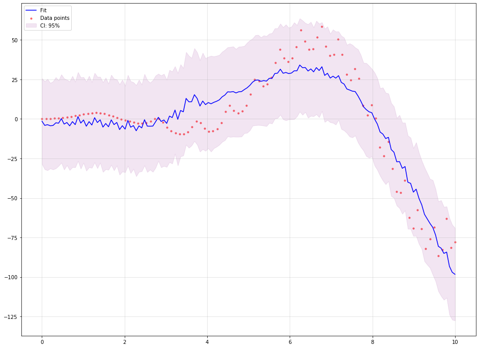
The following example demonstrates how to use GenericRegressor to perform a nonlinear regression based on customized function basis. In the example we use a mixture of polynomials, trigonometric functions and exponential functions of the form \(x^k e^{\pm x/\ell}\) to estimate the function \(x\times e^{\sin(x^2)} + x^2 \times\cos(x)\).
The confidence interval is the default 95% for points:
from random import randint

import matplotlib.pyplot as plt
import numpy as np
from sklearn.linear_model import BayesianRidge

from GeneralRegression.GeneralRegression import GenericRegressor

plt.figure(randint(1, 1000), figsize=(16, 12))

# Make up a 1-dim regression data
n_samples = 100
f = lambda x: x * np.exp(np.sin(x ** 2)) + np.cos(x) * x ** 2
X = np.linspace(0., 10, n_samples).reshape((-1, 1))
y = f(X).reshape((1, -1))[0]


# Function basis generator
def mixed(X, p_d=3, f_d=1, l=1., e_d=2):
    """
    A mixture of polynomial, Fourier and exponential functions

    :param X: the domain to be transformed
    :param p_d: the maximum degree of polynomials to be included
    :param f_d: the maximum degree of discrete Fourier transform
    :param e_d: the maximum degree of the `x` coefficient to be included as :math:`x^d\times e^{\pm x}`

    :return: the transformed data points
    """
    points = []
    for x in X:
        point = [1.]
        for deg in range(1, f_d + 1):
            point.append(np.sin(deg * x[0] / l))
            point.append(np.cos(deg * x[0] / l))
        for deg in range(1, p_d + 1):
            point.append(x[0] ** deg)
        for deg in range(e_d + 1):
            point.append((x[0] ** deg) * np.exp(-x[0] / l))
            point.append((x[0] ** deg) * np.exp(x[0] / (2.5 * l)))
        points.append(np.array(point))
    return np.array(points)


domain = np.linspace(min(X), max(X), 150)

regressor = GenericRegressor(mixed, regressor=BayesianRidge, **dict(p_d=3, f_d=50, l=1., e_d=0))
regressor.fit(X, y)
y_pred = regressor.predict(domain)

plt.scatter(X, y, color='red', s=10, marker='o', alpha=0.5, label="Data points")
plt.plot(domain, y_pred, color='blue', label='Fit')
plt.fill_between(domain.reshape((1, -1))[0],
                 y_pred - regressor.ci_band,
                 y_pred + regressor.ci_band,
                 color='purple',
                 alpha=0.1, label='CI: 95%')
plt.legend(loc=2)
plt.grid(True, alpha=.4)
plt.show()
The output looks like the following image:
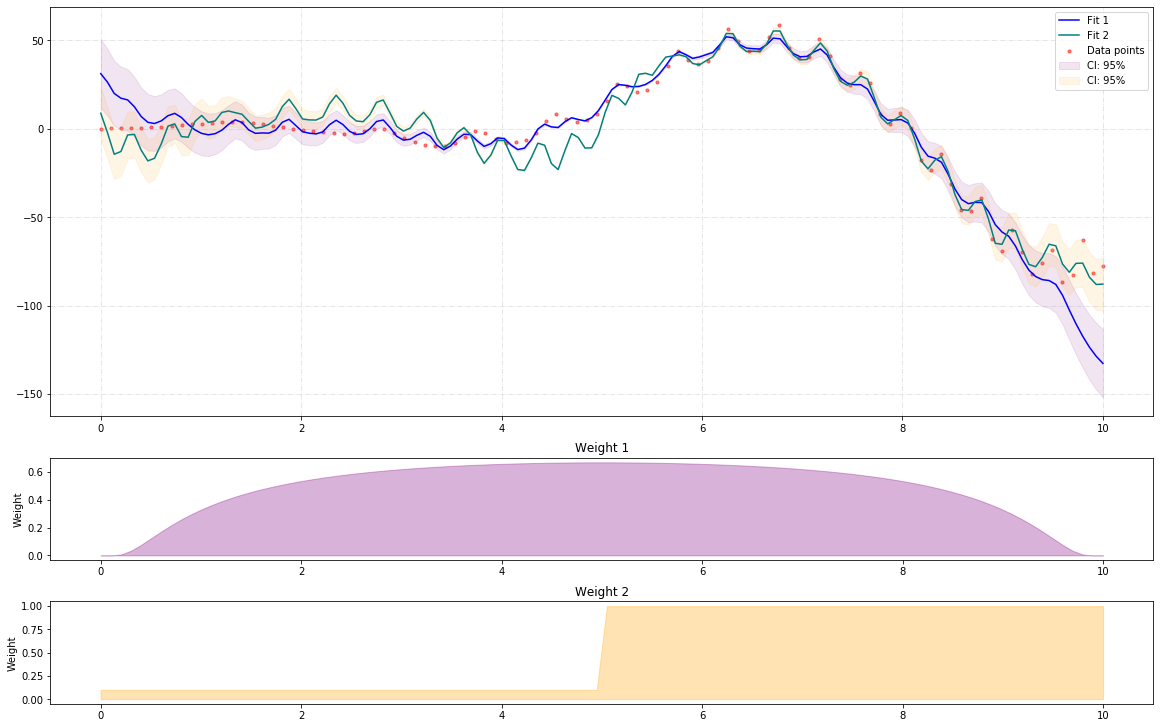
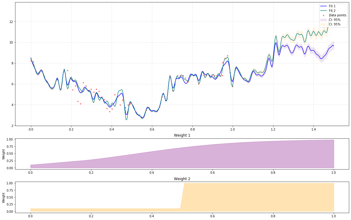
Now, we use two different weights to approximate the same function. The first weight puts more emphasise on the mid points and less on the extreme points, while the second weight puts less emphasise on the lower values and more on the higher ones. This example shows how to use HilbertRegressor and GeneralRegression.extras.FunctionBasis.
In contrast to the previous example, the confidence intervals are 95% defaults for the curves, not the points:
import numpy as np
import matplotlib.pyplot as plt
from random import randint

from GeneralRegression.NpyProximation import HilbertRegressor, Measure
from GeneralRegression.extras import FunctionBasis

plt.figure(randint(1, 1000), figsize=(16, 12))
# Make up a 1-dim regression data
n_samples = 100
f = lambda x: x * np.exp(np.sin(x**2)) + np.cos(x)*x ** 2
X = np.linspace(0., 10, n_samples).reshape((-1,1))
y = f(X)


def pfe_1d(p_d=3, f_d=1, l=1.):
    basis = FunctionBasis()
    p_basis = basis.poly(1, p_d)
    f_basis = basis.fourier(1, f_d, l)[1:]
    e_basis = []
    return p_basis + f_basis + e_basis

domain = np.linspace(min(X), max(X), 150)

x_min, x_max = X.min(), X.max()
x_mid = (x_min + x_max) / 2.
w_min = .1
w_max = 5.
ws1 = {_[0]: np.exp(-1./max(abs((_[0]-x_min)*(_[0]-x_max))/10, 1.e-5))
          for _ in X}
Xs1 = [_[0] for _ in X]
Ws1 = [ws1[_] for _ in Xs1]

ws2 = {_[0]: .1 if _[0] < x_mid else 1.
          for _ in X}
Xs2 = [_[0] for _ in X]
Ws2 = [ws2[_] for _ in Xs2]

meas1 = Measure(ws1)
ell = .7
B1 = pfe_1d(p_d=3, f_d=20, l=ell)

regressor1 = HilbertRegressor(base=B1, meas=meas1)
regressor1.fit(X, y)
y_pred1 = regressor1.predict(domain)

meas2 = Measure(ws2)

regressor2 = HilbertRegressor(base=B1, meas=meas2)
regressor2.fit(X, y)
y_pred2 = regressor2.predict(domain)

fig = plt.figure(randint(1, 10000), constrained_layout=True, figsize=(16, 10))
gs = fig.add_gridspec(6, 1)
f_ax1 = fig.add_subplot(gs[:4, :])
f_ax1.scatter(X, y, color='red', s=10, marker='o', alpha=0.5, label="Data points")
f_ax1.plot(domain, y_pred1, color='blue', label='Fit 1')
f_ax1.plot(domain, y_pred2, color='teal', label='Fit 2')
f_ax1.fill_between(domain.reshape((1, -1))[0],
                 y_pred1 - regressor1.ci_band,
                 y_pred1 + regressor1.ci_band,
                 color='purple',
                 alpha=0.1, label='CI: 95%')
f_ax1.fill_between(domain.reshape((1, -1))[0],
                 y_pred2 - regressor2.ci_band,
                 y_pred2 + regressor2.ci_band,
                 color='orange',
                 alpha=0.1, label='CI: 95%')
f_ax1.legend(loc=1)
f_ax1.grid(True, linestyle='-.', alpha=.4)

f_ax2 = fig.add_subplot(gs[4, :])
f_ax2.set_title('Weight 1')
f_ax2.fill_between(Xs1, [0. for _ in Ws1], Ws1, label='Distibution', color='purple', alpha=.3)
f_ax2.set_ylabel('Weight')

f_ax3 = fig.add_subplot(gs[5:, :])
f_ax3.set_title('Weight 2')
f_ax3.fill_between(Xs2, [0. for _ in Ws2], Ws2, label='Distibution', color='orange', alpha=.3)
f_ax3.set_ylabel('Weight')
The output looks like the following image:
Note
The major code difference between GenericRegressor and HilbertRegressor lies in the way they accept the basis functions. The funcs parameter of GenericRegressor applies the set of basis function on the input points and returns a new set of data points. While HilbertRegressor uses a set of functions as base to perform the required calculations.
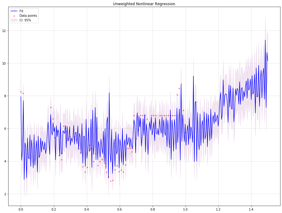
Time series as regression with missing steps
The following example illustrates how a typical time series problem with missing data can be treated as a regression problem while using all existing data points.
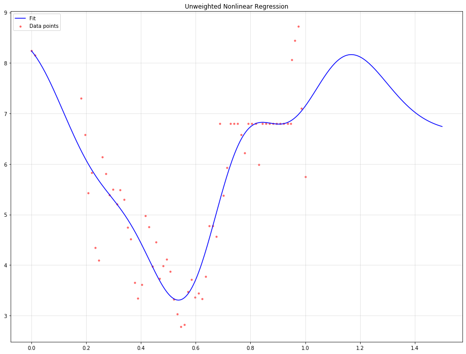
Using unweighted nonlinear regression:
import numpy as np
import matplotlib.pyplot as plt
import pandas as pd
from random import randint
from sklearn.linear_model import BayesianRidge

from GeneralRegression.GeneralRegression import GenericRegressor
from GeneralRegression.extras import Time2Interval

df = pd.read_csv("./data/elec_cost.csv", parse_dates=['Effective Start Date (mm/dd/yyyy)'], infer_datetime_format=True)
dm, dx = df['Effective Start Date (mm/dd/yyyy)'].min(), df['Effective Start Date (mm/dd/yyyy)'].max()
time_trans = Time2Interval(dm, dx)
df['T'] = df.apply(lambda x: time_trans.date2num(x['Effective Start Date (mm/dd/yyyy)']), axis=1)

plt.figure(randint(1, 1000), figsize=(16, 12))

X = df[['T']].values
y = df['Cost'].values

def mixed(X, p_d=3, f_d=1, l=1., e_d=2):
    """
    A mixture of polynomial, Fourier and exponential functions

    :param X: the domain to be transformed
    :param p_d: the maximum degree of polynomials to be included
    :param f_d: the maximum degree of discrete Fourier transform
    :param e_d: the maximum degree of the `x` coefficient to be included as :math:`x^d\times e^{\pm x}`

    :return: the transformed data points
    """
    points = []
    for x in X:
        point = []
        point.append(1.)
        for deg in range(1, f_d + 1):
            point.append(np.sin(deg * x[0] / l))
            point.append(np.cos(deg * x[0] / l))
        for deg in range(1, p_d + 1):
            point.append(x[0] ** deg)
        for deg in range(e_d + 1):
            point.append((x[0] ** deg) * np.exp(-x[0] / l))
            point.append((x[0] ** deg) * np.exp(x[0] / (2.5 * l)))
        points.append(np.array(point))
    return np.array(points)

domain = np.linspace(min(X), max(X)+.5, 300)

regressor = GenericRegressor(mixed, regressor=BayesianRidge, **dict(p_d=5, f_d=50, l=1./12., e_d=-1))
regressor.fit(X, y)
y_pred = regressor.predict(domain)

plt.scatter(X, y, color='red', s=10, marker='o', alpha=0.5, label="Data points")
plt.plot(domain, y_pred, color='blue', label='Fit')
plt.fill_between(domain.reshape((1, -1))[0],
                 y_pred - regressor.ci_band,
                 y_pred + regressor.ci_band,
                 color='purple',
                 alpha=0.1, label='CI: 95%')
plt.legend(loc=2)
plt.grid(True, alpha=.4)
plt.title('Unweighted Nonlinear Regression')
The output would be tha following:
Using weighted nonlinear regression:
import numpy as np
import matplotlib.pyplot as plt
import pandas as pd
from random import randint
from sklearn.linear_model import BayesianRidge

from GeneralRegression.NpyProximation import HilbertRegressor, Measure
from GeneralRegression.extras import FunctionBasis

df = pd.read_csv("./data/elec_cost.csv", parse_dates=['Effective Start Date (mm/dd/yyyy)'], infer_datetime_format=True)
dm, dx = df['Effective Start Date (mm/dd/yyyy)'].min(), df['Effective Start Date (mm/dd/yyyy)'].max()
time_trans = Time2Interval(dm, dx)
df['T'] = df.apply(lambda x: time_trans.date2num(x['Effective Start Date (mm/dd/yyyy)']), axis=1)

plt.figure(randint(1, 1000), figsize=(16, 12))

X = df[['T']].values
y = df['Cost'].values

def pfe_1d(p_d=3, f_d=3, l=1.):
    basis = FunctionBasis()
    p_basis = basis.poly(1, p_d)
    f_basis = basis.fourier(1, f_d, l)[1:]
    e_basis = []
    return p_basis + f_basis + e_basis

domain = np.linspace(min(X), max(X)+.5, 300)

x_min, x_max = X.min(), X.max()
x_mid = (x_min + x_max) / 2.
w_min = .1
w_max = 5.
ws1 = {_[0]: 1./(1. + np.exp(-6*(_[0] - .35)))
          for _ in X}
Xs1 = [_[0] for _ in X]
Ws1 = [ws1[_] for _ in Xs1]
ws2 = {_[0]: .1 if _[0] < x_mid else 1.
          for _ in X}
Xs2 = [_[0] for _ in X]
Ws2 = [ws2[_] for _ in Xs2]
meas1 = Measure(ws1)
ell = 1./12
B1 = pfe_1d(p_d=4, f_d=20, l=ell)

regressor1 = HilbertRegressor(base=B1, meas=meas1)
regressor1.fit(X, y)
y_pred1 = regressor1.predict(domain)

meas2 = Measure(ws2)

regressor2 = HilbertRegressor(base=B1, meas=meas2)
regressor2.fit(X, y)
y_pred2 = regressor2.predict(domain)

fig = plt.figure(randint(1, 10000), constrained_layout=True, figsize=(16, 10))
gs = fig.add_gridspec(6, 1)
f_ax1 = fig.add_subplot(gs[:4, :])
f_ax1.scatter(X, y, color='red', s=10, marker='o', alpha=0.5, label="Data points")
f_ax1.plot(domain, y_pred1, color='blue', label='Fit 1')
f_ax1.plot(domain, y_pred2, color='teal', label='Fit 2')
f_ax1.fill_between(domain.reshape((1, -1))[0],
                 y_pred1 - regressor1.ci_band,
                 y_pred1 + regressor1.ci_band,
                 color='purple',
                 alpha=0.1, label='CI: 95%')
f_ax1.fill_between(domain.reshape((1, -1))[0],
                 y_pred2 - regressor2.ci_band,
                 y_pred2 + regressor2.ci_band,
                 color='orange',
                 alpha=0.1, label='CI: 95%')
f_ax1.legend(loc=1)
f_ax1.grid(True, linestyle='-.', alpha=.4)

f_ax2 = fig.add_subplot(gs[4, :])
f_ax2.set_title('Weight 1')
f_ax2.fill_between(Xs1, [0. for _ in Ws1], Ws1, label='Distibution', color='purple', alpha=.3)
f_ax2.set_ylabel('Weight')

f_ax3 = fig.add_subplot(gs[5:, :])
f_ax3.set_title('Weight 2')
f_ax3.fill_between(Xs2, [0. for _ in Ws2], Ws2, label='Distibution', color='orange', alpha=.3)
f_ax3.set_ylabel('Weight')
The output would be tha following:
And for what it worth
Using support vector regression with rbf:
import numpy as np
import matplotlib.pyplot as plt
import pandas as pd
from random import randint
from sklearn.svm import SVR

from GeneralRegression.extras import Time2Interval

df = pd.read_csv("./data/elec_cost.csv", parse_dates=['Effective Start Date (mm/dd/yyyy)'], infer_datetime_format=True)
dm, dx = df['Effective Start Date (mm/dd/yyyy)'].min(), df['Effective Start Date (mm/dd/yyyy)'].max()
time_trans = Time2Interval(dm, dx)
df['T'] = df.apply(lambda x: time_trans.date2num(x['Effective Start Date (mm/dd/yyyy)']), axis=1)

plt.figure(randint(1, 1000), figsize=(16, 12))

X = df[['T']].values
y = df['Cost'].values

domain = np.linspace(min(X), max(X)+.5, 300)

svr = SVR(kernel='rbf', tol=.0000001, C=10., epsilon=.0001)
svr.fit(X, y)
y_pred = svr.predict(domain)

plt.scatter(X, y, color='red', s=10, marker='o', alpha=0.5, label="Data points")
plt.plot(domain, y_pred, color='blue', label='Fit')
plt.legend(loc=2)
plt.grid(True, alpha=.4)
plt.title('Unweighted Nonlinear Regression')
The output would be tha following: